What are the environmental factors that drive chlorophyll-a (Chl-a) concentration in the Mediterranean Sea?
Study sites
Figure 1 shows the three study sites considered in this work. The first, named Lyon, is located in the Gulf of Lion, between Corsica and Spain. It covers a total area of 14970 km². The Adriatic region, situated between Italy and Croatia, covers a similar area of 14945 km². The third region, Cyprus, is the smallest of the three. It is located south of the island of Cyprus and covers an area of 13352 km².
Data investigation
Figure 2 shows the variation of each response variable and of Chlorophyll-a over time, starting on 1 January 1999. Lyon is the site where Chlorophyll-a is most variable, with a minimum of 0.06 mg m⁻³ and a maximum of 1.41 mg m⁻³. On average, Lyon has a Chla concentration of 0.25 mg m⁻³, which is higher than those of the two other regions: 0.1 mg m⁻³ for Adriatic and 0.04 mg m⁻³ for Cyprus.
Lyon is also the site where the mixed-layer depth (MLD) and nutrients (NO₃, NH₄, and PO₄) show the greatest variability.
Heat flux (HF) and Sea Surface Temperature (SST) vary in the same way regardless of region. The yearly minimum SST in Cyprus is the warmest of all three regions, and overall, the yearly maximum SST is also highest in Cyprus, although it is quite close to the maxima of the other two regions.
Colinearity of variable
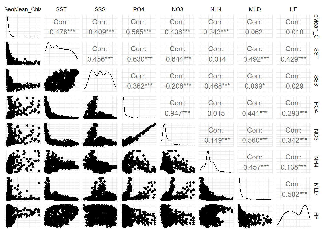
Highly correlated covariates were removed to prevent multicollinearity, which would otherwise inflate parameter uncertainty and obscure the individual ecological effects we aim to quantify. As shown in Figure 3, PO₄ and NO₃ are almost perfectly correlated (R = 0.997). NO₃ is also strongly correlated with NH₄ (R = 0.77), and PO₄ with NH₄ (R = 0.742). Therefore, individual nutrient concentrations were excluded from the analysis. Instead, we included two derived variables:
\[ NPratio = (NO3+NH4)/PO4 \]
&
\[ TotalNutrient = PO4+NO3+NH4 \] These aggregated metrics provide more interpretable and independent representations of nutrient availability and stoichiometry (Figure 4).
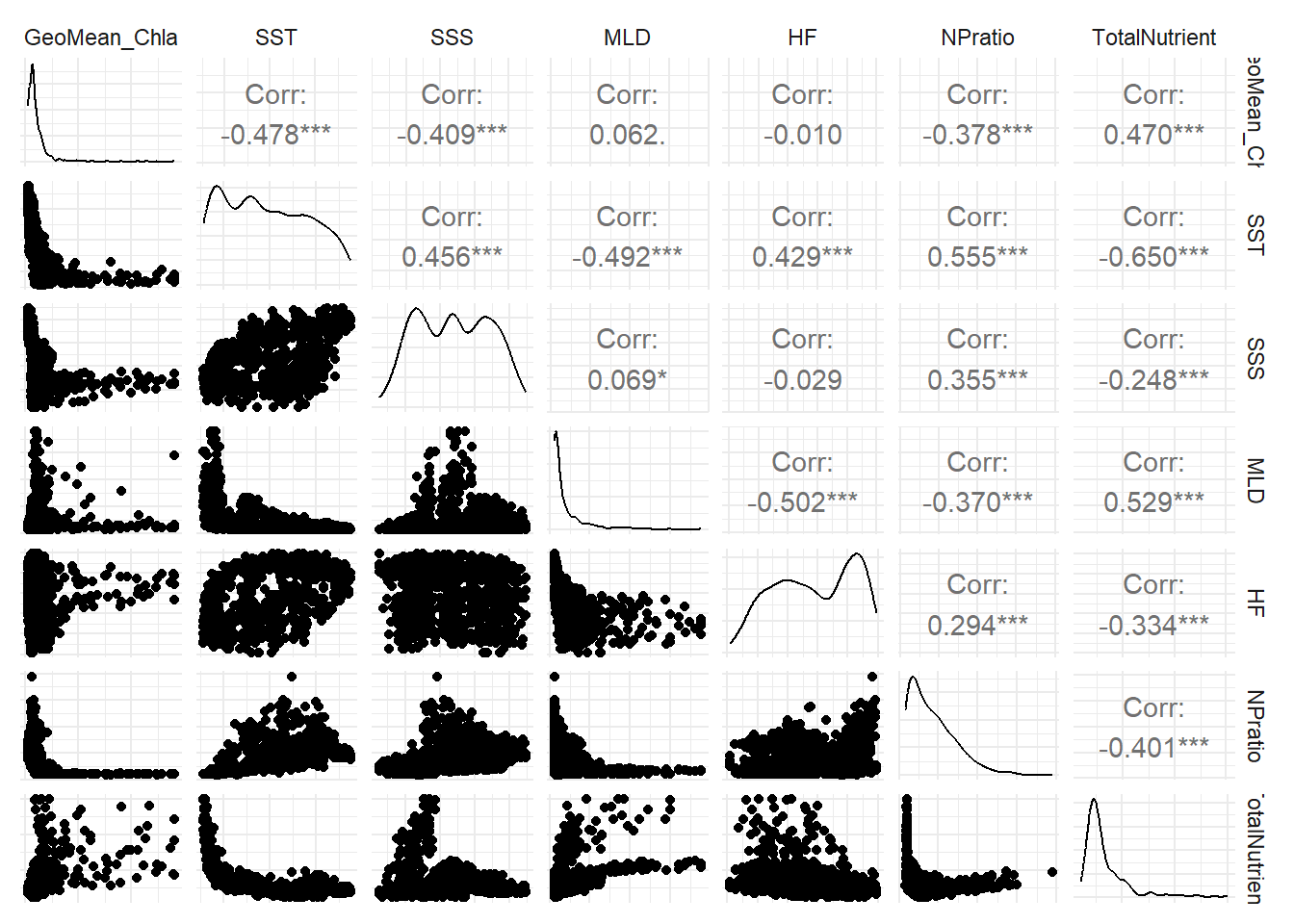
As a result of the variable selection process, chlorophyll-a concentration will be modeled as a function of sea surface temperature (SST), sea surface salinity (SSS), mixed layer depth (MLD), heat flux (HF), nutrient stoichiometry (NP ratio), and total nutrient availability (TotalNutrient).
Model Building
We fitted a Bayesian Generalised Additive Model (GAM) with a Gamma response in brms (Bürkner 2017, 2018, 2021) to explain the geometric-mean chlorophyll-a concentration (GeoMean_Chla) in for each of the 3 sites (one model for each site).
The response (GeoMean_Chla) is strictly positive and right-skewed, therefore we adopted a Gamma distribution with a log link (See equation below). Six environmental drivers, likewise available as monthly means, were entered as thin-plate regression splines to allow non-linear effects: sea-surface temperature (SST), sea-surface salinity (SSS), the nitrogen-to-phosphorus ratio (NPratio), summed dissolved nutrients (TotalNutrient), mixed-layer depth (MLD) and the Heat flux (HF). All predictors were centred and scaled prior to modelling. Weak but regularising priors were used: Student-t(3, 0, 2.5) for the intercept, half-Student-t(3, 0, 2.5) for each smooth’s standard deviation, and Gamma(0.01, 0.01) for the Gamma shape parameter φ. Posterior inference relied on the NUTS Hamiltonian Monte-Carlo sampler with 4 chains × 10 000 iterations, discarding the first 1 000 iterations of each chain as warm-up. Convergence and sampling quality were verified by inspecting the Gelman–Rubin statistic (Rhat ≤ 1.01 for every parameter) together with bulk and tail effective sample sizes (all > 5 000), confirming that the posterior was thoroughly explored and free of divergent transitions.
\[\begin{aligned} \mathrm{GeoMean\_Chla}_{i} &\sim \mathrm{Gamma}\!\bigl(\mu_{i}\,\varphi,\;(1-\mu_{i})\,\varphi\bigr) \\[6pt] \log \mu_{i} &= \eta_{i} \\[4pt] \eta_{i} &= \alpha + f_{1}(\mathrm{SST}_{i}) + f_{2}(\mathrm{SSS}_{i}) + f_{3}(\mathrm{N{:}P}_{i}) + f_{4}(\mathrm{SumNutri}_{i}) + f_{5}(\mathrm{MLD}_{i}) + f_{6}(\mathrm{HF}_{i}) \\[8pt] f_{j}(x) &= \sum_{k=1}^{K_{j}} \beta_{jk}\,B_{jk}(x), \qquad j = 1,\dots,6 \\[10pt] \alpha &\sim t_{3}(0,\,2.5) \\[2pt] \beta_{jk} &\sim \mathcal N\!\bigl(0,\,\sigma_{j}^{2}\bigr) \\[2pt] \sigma_{j} &\sim t^{+}_{3}(0,\,2.5) \\[2pt] \varphi &\sim \mathrm{Gamma}(0.01,\,0.01) \end{aligned}\]